Optional Practical: Ripple tank simulation (GeoGebra)
Introduction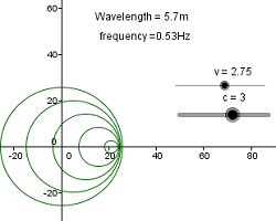
In this exercise 2D waves will be simulated in GeoGebra by drawing a sequence of circles that expand at a constant rate, these circles represent wavefronts from a wave progressing from a point source.
Note: This worksheet assumes some knowledge of the basic tools in GeoGebra.
Drawing circles
Circles can be plotted by inputting the equation of a circle or using the circle function.
- Input Circle[(0, 0), 5]
You will now have a circle with centre at the origin with radius 5.
- Make a slider t representing time from 0 to 10 increment 0.01
- Double click the circle and replace [(0,0),5] with [(0,0),t]
- Right click the t slider and turn animation on.
The radius of the circle will now increase at a constant rate
- Add a slider c representing the wave velocity from 0 to 5 increment 0.01
- Double click the circle and replace t with ct
- The speed at which the circle propagates can now be controlled with the c slider.
Using Sequences
To make a sequence of waves you could manually add lots of circles that start at different times but it’s much easier with the “sequence” function. First let’s see how this work by plotting a series of points.
- Input “sequence” and choose
Sequence[
- Replace the <> terms with Sequence[(i, 0), i, 0, 50, 5]
To make a series of circles:
- Input Sequence[Circle[(0, 0), i], i, 0, 50, 5]
To give the circles expanding radius
- Input Sequence[Circle[(0, 0), c (t - i)], i, 0, t, 1]
This draws a circles at 1s intervals with radius = c(t-i) substituting numbers will help to understand this let’s say c = 2:
t = 0s – the End value is 0 so no circled drawn
t = 1s – End value = 1 so i = 1 radius of circle = c(1-1) = 0
t = 2s – End value = 2 so I = 1 and i = 2 circle drawn with radii 0 and 2(2-1) = 2
t = 3s – End value = 3 so I = 1,2,3 circles drawn with radii 0,2,4 etc.
To vary the time period of the wave
- Add a slider T from 0 to 5 increment 0.01
- Change Sequence[Circle[(0, 0), c (t - i)], i, 0, t, 1]
- Run the animation and see the effect of changing T and c
- The frequency of the wave = 1/T, input the equation f=1/T and display it by adding text
- The wavelength = cT, input the equation λ = cT and display.
Investigation
- Make a second wave with centre (0,5) and investigate the interference effect.
- Make a slider so you can adjust the separation of the sources.
Doppler Effect
The Doppler effect is the change in frequency caused by the relative motion of source and observer, here we will move the source.
- Add a slider v representing the source velocity from 0 to 5 increment 0.01.
- Change the wave sequence to Sequence[Circle[(v i, 0), c (t - i)], i, 0, t, T]
This will change the position of the centre for each successive values of i
Investigation
- Try changing v and c to see how the wave pattern changes.
- For chosen values of c and v stop the animation and measure the wavefront on either side of the source.
- Calculate the frequency of the observed waves and compare with the result given by the equations in the text book.

Multiple sources
Before moving on to this exercise it might be worth starting again with a blank project
To make multiple sources you can use the sequence function on a sequence. To make line of wave sources with separation s and width w:
- On your new GeoGebra file recreate the sliders o
- Add sliders for s (0 to 1 increment 0.0001) and w (0 to 20 increment 0.0001)
- In options set rounding to 4 dp
- Sequence[Sequence[Circle[(0, k), c (t - i)], i, 0, t, T], k, 0, w, s]
- Don't animate these examples as it will probably cause your computer to crash, just set t = 10.
- Set c = 0.1
- Hide the sliders for c and t.
- Write an equation for λ and display on your graph.
- Vary sliders T, s and w to see how the change the pattern.
Huygens construction
- Set w = 20, λ = 0.2, s = 0.2
Observe how the wavelets add to give wavefronts.
- Vary the sliders and observe what happens.
Single slit diffraction
Single slit diffraction can be modeled by considering a large number of wavelets across a narrow slit. The maxima are the light parts, this is where the lines are overlapping leaving the background visible.
- Set the line thickness to 1 in properties.
- Set λ = 0.0175, s = 0.005 and w = 0.06
- Vary these parameters and observe what happens.

Diffraction grating
A diffraction grating can be modeled by a large number of evenly spaced wavelet sources.
- Set λ = 0.04, s = 0.06 and w = 0.3
- Vary the parameters and observe the effect.