Plotting a curve

So far LoggerPro has been used to plot the points from an experiment, the next step is to plot the curve that fits these points. LoggPro will join these points dot to dot but this is not what we want so first remove this by double clicking the graph and unchecking the box next to "connect points". To make the points stand out you can check the box next to "point protectors".

You will now have a graph with points on it but no line. You could get the computer to simply draw a smooth curve through the points but that we want to know the equation of the line so that wouldn't be much use. In this course we will be using the graph to support a theoretical relationship or find an unknown value. In this example we predict that the rate of change of temperature is inversley proportional to the mass of water so we expect that ΔT and m is are inversley proportional. This means that the smooth curve joining the dots will have the function ΔT = k/m where k is a constant. (we know that P = mcΔT/Δt so ΔT = PΔt/c x 1/m so the constant is PΔt/c). Loggerpro will find the bestfit curve for the data.

To plot a curve first press the curve fit button this will open a dialogue box like the one below.

There are a lot of curve fit options in loggerPro but there is no point in simply trying to find which one fits without knowing the physical significance of the equation. By applying theory we expect that ΔT is proportional to 1/m so we will plot a y=1/x curve. This is A/m or [inverse] in loggerPro, choose this option from the menu and click "try fit" followed by "OK". You will now have a best fit curve with the equation displayed on the graph as shown below.

Error Bars

Because of uncertainties in the data the line does not pass through all the data points, the standard way of showing the uncertainty in each point is to add error bars to the graph. How to estimate uncertainties is outlined in the section on uncertainties, for this example we will assume that the uncertainty in ΔT is ±0.5°C and the uncertainty in m is 0.01kg. To plot error bars simply double click the header in the column, this will open the graph options dialogue box, if you click the "options" tab you will open the box below.

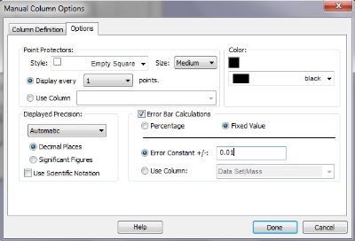
Check the "error bar calculation box" and the "fixed value" then fill in the value for the error (0.01 for mass and 0.5 for ΔT) when you close this dialogue box the eror bars will appear on your graph as below.